14 Jun 2026
Introduction
In this post, I recreate a model of an evolutionary game put forward by mathematical finance researchers in 2009. Their work suggests that, in systems where participants interact with one another to affect the probability of future outcomes, it can take a long time for steady state behavior to emerge. This has interesting implications for financial markets. For example, the interaction between hedge fund strategies can result in inefficencies that persist for significantly longer than the Efficient Markets Hypothesis would suggest is possible. In the second half of the post, I extend their model slightly to see if the qualitative behavior persists.
First, some background on how I found the paper and why I found it so compelling.
Background
I’ve been working my way through a recommended reading list for those interested in quantitative trading by Kris Abdelmessih, a former options trader at SIG who writes the Moontower substack. So far I’ve read Howard Marks’ The Most Important Thing, Agustin Lebron’s The Laws of Trading, and Annie Duke’s Thinking in Bets. I actually read another one of Annie Duke’s books, Quit: The Power of Knowing When to Walking Away, a few years ago - her books are great reads.
The impetus for this post came from the list entry I’m currently reading, Andrew Lo’s Adaptive Markets. It’s my favorite so far because it connects the mathematical biology I studied in undergrad with mathematical finance in surprising ways. Chapter 8’s discussion of market efficiency introduces J. Doyne Farmer, a polymath researcher who has contributed to chaos theory, biology, and mathematical research in addition to founding one of the first quantitative hedge funds, Prediction Company.
Lo cites a 2009 paper by Dmitriy Cherkashin, J. Doyne Farmer, and Seth Lloyd in support of the claim that market inefficiencies can persist for significant periods of time due to the interaction of trading strategies in the market. He draws an analogy to the Lotka-Volterra equations, a predator-prey model illustrating how population sizes can oscillate over time rather than reaching a single fixed point.
I ran into the Lotka-Volterra equations for the first time in Darren Wilkinson’s textbook, Stochastic Modeling for Systems Biology. The interaction between predators and prey introduces relatively simple non-linear terms, which, for the right initial conditions, lead to oscillating populations of both predator and prey. The predators depend on the prey in order to eat and be able to reproduce; however, as the predators eat their prey, they drive the prey population down and the predator population up until there aren’t enough prey for the predators to survive and reproduce. At this point, the predator population decreases enough for the prey population to stabilize and grow. The cycle repeats infinitely. Doyne drew an analogy with hedge funds, where the interaction of market participants leads to boom and bust cycles for different strategies.
Returning to Cherkashin et. al.: their 2009 paper builds a simple betting game to show that interactions between strategies can cause inefficiencies to persist for long periods of time. They provide simulation data illustrating this behavior as well as an analytical breakdown of how the math leads to this behavior.
Part One: Recreating Their Results
Introduction & Notation
The paper proceeds by setting up an evolutionary game called (rather fancifully) the Reality Game. They provide a general framework but focus on a coin flip where the probability of heads at each time step is determined by a function of the prior outcome referred to as the reality map. Players bet all of their wealth each round with no house take, and the winners receive a portion of the total pool relative to what they bet on the winning outcome (i.e., pari-mutuel betting).
Here’s some notation from the paper:
- $N$ agents place wagers on $L$ possible outcomes. For a coin toss, $L=2$.
- $s_i$ is the amount of player $i$’s total wealth he or she wagers on heads (so, $1-s_i$ is their wager on tails).
- $w_i$ is the portion of the total wealth pool that player $i$ holds. Wealth is normalized so $\sum_i w_i = 1$.
- $p = \sum_i s_i w_i$ is the total amount bet on heads. Of course, $1-p$ is the total bet on tails.
- Supposing heads wins, $\pi_i = \frac{s_i w_i}{p}$ is the payout to player $i$. if tails wins, $\pi_i = \frac{(1-s_i)w_i}{1-p}$ is the payout.
- $q$ is the probability that heads wins. The reality map is the function $q(p)$.
Here’s an interesting aside: if $q$ is a constant, the wealth updating rule is analogous to Bayesian inference. In the below, the subscript $\lambda$ refers to the winner of either heads or tails. So, $p_{\lambda} = p$ when heads wins and $1-p$ when tails wins.
\[w_i^{(t+1)} = \frac{s_{i\lambda} w_i^{(t)}}{p_{\lambda}}\]You can interpret the prior period wealth as the prior probability of heads and the next period wealth as the posterior probability. Just as Bayesian inference leads to more and more accurate estimates of the true probability distribution, this model causes players who probability match (i.e., they bet on each outcome proportionally to its probability) to eventually accrue all of the wealth.
More generally, reality maps are characterized according to how they vary with $p$:
- Objective, where $q(p) = const.$. Previous results don’t affect the future probability of the game.
- Self-defeating, where $q’(p) < 0$. The more wealth bet on heads, the less likely it becomes in the next round.
- Self-reinforcing, where $q’(p) > 0$. The more wealth bet on heads, the more
likely it becomes in the next round.
- The special case of $q(p) = p$ is referred to as purely subjective, i.e., the future probability of heads is exactly equal to what was previously bet on heads.
The Simulation
Using the notation defined above, it’s pretty simple to write a function which simulates rounds of betting. I follow the paper’s example of using 29 strategies evenly spaced over $[0,1]$, where a strategy is just a value for $s_i$, the portion of wealth bet on heads. The function returns the wealth distribution and the values of the reality map over time.
import random
import numpy as np
import matplotlib.pyplot as plt

def simulations(N, T, realityMap):
    # N is the number of strategies, evenly spaced over [0,1]
    # T is the number of rounds to simulate
    # realityMap is the reality map, a function defining q

    # define strategies
    strategies = np.arange(1,N) / N

    # store wealth for each strategy
    wealth = np.zeros([T,N-1])
    wealth[0] = np.ones(N-1) / (N-1)

    # Initiate reality map
    q = np.zeros(T)
    q[0] = 0.5

    for i in range(1,T):
       # Calculate outcome
       outcome = random.random() < q[i-1]

       # Update Wealth
       betOnHeads = sum(strategies * wealth[i-1])
       if outcome:
           wealth[i] = [strategies[j] * wealth[i-1][j] for j in range(0,N-1)] / betOnHeads
       else:
           wealth[i] = [(1-strategies[j]) * wealth[i-1][j] for j in range(0,N-1)] / (1-betOnHeads)

       # update reality map
       q[i] = realityMap(betOnHeads)

    return q, wealth
The paper uses a family of arctangent-based functions for the reality maps, along with simple self-defeating and self-reinforcing examples. They chose that set of functions because it has a single parameter to control the degree of objectivity / self-reinforcement. The set of functions used in figure 1 are below:
# figure (a)
def selfDefeatingRM(p):
    return 1-p

# figure (b)
def figBRM(p):
    return 0.5 + np.arctan((np.pi * 0.5 * (p - 0.5))/(1 - (2*p - 1)**2)) / np.pi

# figure (c)
def subjectiveRM(p):
    return p

# figure (d)
def figDRM(p):
    return 0.5 + np.arctan((np.pi * 1.5 * (p - 0.5))/(1 - (2*p - 1)**2)) / np.pi

# figure (e)
def multiModalRM(p):
    return (3 * p) % 1
Results & Graphs
With our simulation function and the reality maps defined, we can recreate their Figure 1 showing how the reality maps $q(p)$ evolve.
# Run and plot the simulations

fig = plt.figure()
gs = fig.add_gridspec(2,6)

# Row 1
ax_a = fig.add_subplot(gs[0, 0:2])
ax_a.set_title("1a (Self-Defeating)")
ax_a.set_ylim([0,1])

ax_b = fig.add_subplot(gs[0, 2:4], sharey=ax_a)
ax_b.set_title("1b (alpha = 0.5)")

ax_c = fig.add_subplot(gs[0, 4:6], sharey=ax_a)
ax_c.set_title("1c (Pure Subjective)")

# Row 2
ax_d = fig.add_subplot(gs[1, 1:3], sharey=ax_a)
ax_d.set_title("1d (alpha = 1.5)")

ax_e = fig.add_subplot(gs[1, 3:5], sharey=ax_a)
ax_e.set_title("1e (Multi-Modal)")

x = np.arange(0,2000)
x_e = np.arange(0,10_000)

for i in range(0,30):
    a_q, a_wealth = simulations(30, 2000, selfDefeatingRM)
    b_q, b_wealth = simulations(30, 2000, figBRM)
    c_q, c_wealth = simulations(30, 2000, subjectiveRM)
    d_q, d_wealth = simulations(30, 2000, figDRM)
    e_q, e_wealth = simulations(30, 10_000, multiModalRM)

    ax_a.plot(x,a_q)
    ax_b.plot(x,b_q)
    ax_c.plot(x,c_q)
    ax_d.plot(x,d_q)
    ax_e.plot(x_e,e_q, linewidth=0.1, linestyle='dotted')

plt.tight_layout()
plt.show()
In the figures below, the x-axis is the number of rounds that have been played and the y-axis is the value of $q(p)$. The different colored lines represent different simulation instances.
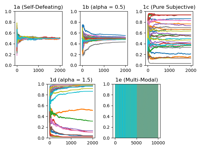
My results match the qualitative behavior shown in the paper. (a) and (b) show the probability moving towards the fixed point $q(p) = 0.5$, more quickly in (a) than in (b). For (a), the only fixed point for $q(p)$ is 0.5, but (b) also has 0 and 1. Because (b) is only weakly self-reinforcing the early round fluctuations in wealth aren’t enough to push $q(p)$ towards 0 or 1.
Skipping ahead to (d), the stronger self-reinforcing reality map leads to larger early fluctuations which push $q(p)$ towards 0 or 1. The total wealth moves more quickly towards either those who bet more on heads or those who bet more on tails. Sometimes the convergence is very slow, like the orange line and dark green lines in the center of the graph.
(c) is interesting - the steady state is determined by the first several dice rolls, as they shift wealth towards a particular probability of heads which quickly cements itself as wealth concentrates in the strategies near that probability. In the purely subjective case, after a few rounds one of the players will amass enough of the wealth that they get to effectively shape reality - they command so much of the wealth that their strategy becomes the fixed point.
Its worth ruminating on the fact that in all of these scenarios, wealth concentrates one just one strategy. Once a particular player has a large portion of the wealth, their bets make up a large portion of the pot, so it’s very unlikely for them to go on a losing streak long enough to unseat them.
My multi-modal graph is difficult to read; I tried reducing the line width and making it dotted to make it easier, but the wild oscillations between 1 and 0 give a result a bit like when I tried to mix paints in first grade - it just comes out muddy and unclear. Looking under the hood, however, I’m seeing the same behavior the paper reported. Wealth becomes concentrated at strategies $s = 1/3$ and $s = 2/3$, the discontinuities in the reality map.
Part Two: Simple Extension
What if instead of a binary outcome (i.e., a coin toss), we had several possible outcomes? I used Cherkashin et. al.’s framework to develop a similar set of simulations, but for a dice roll.
Before jumping into this, I should explain why I did this. I didn’t think the extension would disagree with the paper’s results or even provide new results worth mulling over. Rather, this was a way to make sure I really understood the paper’s set up and central conjectures. It’s one thing to just read it and think about it, and a whole other thing to do some original work based on it.
In high school, my chemistry teacher told us that to really learn something we needed to encounter it multiple times in multiple formats. Read the textbook, listen in class, do your homework, study for the test, and then take the test. This is a good framework to which I’d add that one of those formats should take the form of original exploration. Even a trivial extension on the material will force you to grapple with the minutiae of whatever it is you’re studying.
Notation
Here’s our updated notation:
- $N$ agents place wagers on $L$ possible outcomes. Here, $L=6$.
- $s_{il}$ is the amount of player $i$’s total wealth he or she wagers on the $l$th outcome. $s_i$ is now a vector with dimension $L$.
- $w_i$ is the portion of the total wealth pool that player $i$ holds. Wealth is normalized so $\sum_i w_i = 1$.
- $p_l = \sum_i s_{il} w_i$ is the total amount bet on outcome $l$.
- Player $i$ gets a payout of $\pi_{i\lambda} = \frac{s_{i\lambda} w_i}{p_{\lambda}}$ when outcome $\lambda$ wins.
- $q_l$ is the probability that outcome $l$ wins. $q$ is now a vector with dimension $L$. The reality map is the vector-valued function $q(p)$.
We’ll need to keep in mind the dimensions of our vectors when we write the simulation function.
Setting the Strategies
The paper uses 29 strategies evenly spaced over the space of probabilities of heads. I wanted the strategies for this extension to also be evenly spaced in some sense. To accomplish that, I wanted the following to be true:
- Each player puts at least some money on each outcome;
- Each player puts a different amount of money on each outcome; and
- Overall, the strategies should be balanced between all the players so that there’s an equal amount of money being put on each outcome in the first round.
To accomplish this, I set the strategies as all the possible orders of the
numbers 1 - 6, divided by the sum of the range from 1 to 6 (which is 21). There
are $6! = 720$ such strategies. Here’s the code, using the itertools package
to get all the possible permutations:
import itertools

# define strategies
L = np.arange(1,7)
strategies = np.asarray(list(itertools.permutations(L))) / 21
Simulation Function
The simulation function is pretty similar, but because there are more than two outcomes, everything’s a vector now. It’s a good excuse to practice our linear algebra.
import random
import numpy as np
import matplotlib.pyplot as plt
import matplotlib.animation as animation
import itertools

def simulations(T, realityMap):
    # T is the number of rounds to simulate
    # realityMap is the reality map, a function defining q

    # define strategies
    L = np.arange(1,7)
    strategies = np.asarray(list(itertools.permutations(L))) / 21

    # N is the number of strategies
    N = strategies.shape[0]

    # store wealth for each strategy
    wealth = np.zeros([T,N])
    wealth[0] = np.ones(N) / N

    # Initiate reality map
    q = np.zeros([T, 6])
    q[0] = np.ones(6) / 6

    for i in range(1,T):
       # Calculate outcome
       roll = random.choices(L, weights=q[i-1])[0]
       outcome = np.zeros(6)
       outcome[roll-1] = 1

       # Update Wealth
       s_lambda = strategies @ outcome # 720-by 6 * 6-by-1 = 720-by-1
       p_lambda = np.dot(s_lambda, wealth[i-1]) # integer value

       wealth[i] = (np.eye(N) * s_lambda) @ wealth[i-1] / p_lambda

       # update reality map
       # p is the amount bet on each strategy (6 by 1 vector)
       p = strategies.T @ wealth[i-1]
       q[i] = realityMap(p)

    return q, wealth
Where before we had an array, we now have an array of vectors, and where before
we had a single value, we have a vector of values. I use the @ symbol to
multiply strategies, which can be viewed as a 720-by-6 matrix, by the
outcome unit vector, which gives us $s_{\lambda}$. Similarly, $p_{\lambda}$
is the dot product of $s_{\lambda}$ and $w$.
I’m pleased with how I updated player wealth: by casting $s_{\lambda}$ to a diagonal matrix, we can multiply it by the previous round’s wealth and normalize it by $p_{\lambda}$. The division happens entry-by-entry, so the total wealth still sums to one.
Defining the Reality Maps
To keep things simple, I only used the pure self-defeating and pure subjective reality maps for this extension. Numpy handles arrays very neatly, so the reality map functions don’t need much updating. The subjective map remains the same, and the self-defeating map just needs to be normalized for the number of possible outcomes.
Suppose we have a vector $x$ such that $\sum_i^n x_i = 1$. We can “invert” each of the entries by subtracting them from one, but if we stop there, the new sum is $\sum_i^n 1 - x_i = \sum_i^n 1 - \sum_i^n x_i = n - 1$. We can normalize our new vector by dividing every entry by $n-1$. If that’s not immediately obvious, you can let $a$ be the normalizing constant and solve for it like below:
\[\sum_i^n x_i = 1 \\ \sum_i^n \frac{1-x_i}{a} = 1 \\ \frac{1}{a}(\sum_i^n 1 - \sum_i^n x_i) = 1 \\ \frac{1}{a}(n - 1) = 1 \\ a = n - 1\]Here’s the code:
# define our reality maps
def selfDefeatingRM(p):
    return (1 - p) / (len(p)-1)

def subjectiveRM(p):
    return p
Results & Graphs
I simplified the graphing a bit below, and created an animation for the reality maps $q$. Below is the code, followed by a gif of the animation.
# Run and plot the simulations

fig, axs = plt.subplots(nrows=1, ncols=2, sharey='all')
x = np.arange(0,6)
T = 1_000 # number of rounds

axs[0].set_title("Self-Defeating")
axs[1].set_title("Purely Subjective")

axs[0].set_xticks(x)
axs[1].set_xticks(x)
axs[0].set_xticklabels(np.arange(len(x))+1)
axs[1].set_xticklabels(np.arange(len(x))+1)

axs[0].set_ylim(0,0.5)

sd_q, sd_wealth = simulations(T, selfDefeatingRM)
sub_q, sub_wealth = simulations(T, subjectiveRM)

sd_graph = axs[0].bar(x, sd_q[0])
axs[0].axhline(y=0.16666, color='r', linestyle='--')

sub_graph = axs[1].bar(x, sub_q[0])
axs[1].axhline(y=0.16666, color='r', linestyle='--')

# Animate
def animate(i):
    y_sd = sd_q[i]
    y_sub = sub_q[i]
    for i, b in enumerate(sd_graph):
        b.set_height(y_sd[i])
    for i, b in enumerate(sub_graph):
        b.set_height(y_sub[i])

anim = animation.FuncAnimation(fig, animate,
                               repeat=False, blit=False, frames=T, interval=50)

anim.save('dice_roll.gif')
The red dashed line indicates even $\frac{1}{6}$ probabilities for each outcome.
As expected, this extension behaves exactly how the coin toss version of the model would predict.
The self-defeating map has a fixed point for $q(p)$ where the probability of each outcome is equal. The map hovers around that point in the gif above. My set up of the strategies means that no one player is betting exactly even amounts on each outcome, so unlike before, the wealth does not concentrate on a single player. Were we to introduce a rational player (as Cherkashin et. al. do), they would be able to eventually capture most of the wealth.
The pure subjective map is all fixed points, and shows much more fluctuation early on before settling out at one of the strategies, which as before, accumulates the lion’s share of the wealth. A key characteristic of the subjective case is that wealth accumulation leads to less volatility in the reality map.
Conclusion
Cherkashin et. al. go on to provide an analytic treatment of the game, showing that the approach to an equilibrium obeys a power law, and that the behavior is different when that equilibrium is not at one of the endpoints (0 or 1). They also introduce a rational, utility-maximizing player, the design of which is fascinating in itself. The key insight for understanding markets is that, early on when wealth isn’t concentrated and the oscillations in the reality map are larger, a rational player can make considerable profits. Those profits dwindle as the reality map approaches an equilibrium point.
The paper is worth a read for those of you interested in the self-reinforcing nature of markets. The authors suggest several future lines of inquiry bringing their game closer to real life markets in nature. This is the kind of thing that I love about applied math: the process of tweaking and expanding a model to make it more and more useful. It’s easy for me to enter a flow state playing around with these things, and the way your interpretations lead immediately to possible extensions is really exciting.
To end on a personal note, I’ve got about a month and a half until I start the Master in Computational Finance program at Carnegie-Mellon. Hopefully going back to school will mean getting to do a lot more stuff like this.