The Code
After a long break, I’ve finally gotten back to my amortizing bond model investigation. The previous posts give the background on what I’m trying to accomplish here: let’s jump right in to the code.
import numpy as np
from sympy import *
import pickle
import dill
import matplotlib.pyplot as plt

np.set_printoptions(formatter={'float':'{:,.4f}'.format})
%matplotlib widget

# R is the annual revenue constraint
# r is the coupon rate
# g is the annual revenue growth rate
R, r, g = symbols('R r g')

# Parameters
# Maturities is the maturities we're testing
# Coupons is the coupon rates we're testing
# GrowthRates is the growth rates we're testing
Maturities = np.arange(10,41,1)
Coupons = np.arange(0.02,0.125,0.0025)
GrowthRates = np.arange(0.0,0.06,0.01)

# This lambda expression makes it easier to fill in the revenues
growth_rate = lambda i, n : (1+g)**i

# Generate the expressions for the first year's principal
FirstYrPrincipal = Matrix(np.zeros([len(Maturities)]))

for i, maturity in enumerate(Maturities):
    A = Matrix((1+r) * np.eye(maturity) + r * np.triu(np.ones([maturity,maturity]),1))
    revenue = Matrix(np.fromfunction(lambda j: growth_rate(j, maturity) * R, shape=(maturity,), dtype=float))
    FirstYrPrincipal[i] = A.solve(revenue)[0]
Generating all of those expressions is computationally expensive. It took my M2 Mac Mini about 11 minutes to run the code up to here. I used the Pickle and Dill libraries to save down the expressions as both Python objects and functions. By default, the functions save everything into the present working directory. The code for saving / loading the expressions is below.
# Save the expressions with Pickle
with open('FirstYrPrincipal.pkl', 'wb') as f:
    pickle.dump(FirstYrPrincipal, f)
# Save them as functions with Dill
PrincipalFunctions = lambdify((R, r, g), FirstYrPrincipal, 'numpy')
with open('PrincipalFunctions.dill','wb') as f:
    dill.dump(PrincipalFunctions, f)
# Load in the functions
with open('PrincipalFunctions.dill','rb') as f:
    PrincipalFunctions = dill.load(f)
Now that we have all of our symbolic expressions, we can calculate the first year’s principal amount for each maturity, coupon, and growth rate. As a reminder, a negative calculated first year principal indicates that the bond model doesn’t pencil for the parameters - that is, we can’t have a fully amortizing bond model with this combination of maturity, coupon, and growth rate. You can think of a negative calculated principal amount as meaning the issuer would need to borrow funds in that year to pay interest on the principal due in later years. There is a workaround for this we’ll discuss later.
# Calculate everything

results = np.zeros([len(Maturities),len(Coupons),len(GrowthRates)])

for j, coupon in enumerate(Coupons):
    for k, growth in enumerate(GrowthRates):
        principals = PrincipalFunctions(1000000, coupon, growth)
        for i, values in enumerate(principals):
            results[i][j][k] = values.item()
Below, I create a slideshow of graphs showing when we get a negative first principal payment for different maturities, coupon rates, and growth rates. The slider lets you change the growth rate assumption. I played around with 3D visualizations, but they were all much clunkier to interpret.
# We'll create a new array with boolean values indicating whether the first
# principal payment is zero
ZeroPrincipals = results < 0

# The Graph
from matplotlib.widgets import Slider

fig, ax = plt.subplots()
plt.subplots_adjust(bottom=0.25) # makes room for slider
initial_slice = ZeroPrincipals.shape[2] // 2 # midpoint of our growth axis
img = ax.imshow(ZeroPrincipals[:, :, initial_slice], cmap='coolwarm', origin='lower')

plt.ylabel("Maturity (years)")
plt.xlabel("Coupon (percentage)")

coupon_labels = [f"{v*100:.0f}%" for v in Coupons]
coupon_indices = np.arange(len(Coupons))
plt.xticks(ticks=coupon_indices[0::4], labels=[coupon_labels[i] for i in coupon_indices[0::4]])

mat_labels = [f"{v:.0f}" for v in Maturities]
mat_indices = np.arange(len(Maturities))
plt.yticks(ticks=mat_indices[0::5], labels=[mat_labels[i] for i in mat_indices[0::5]])

plt.grid(visible=True, color='white', linestyle='--', linewidth=0.5, alpha = 0.7)

ax_slider = plt.axes([0.25, 0.1, 0.5, 0.03]) # Just places the slider on the plot
slice_slider = Slider(
    ax=ax_slider,
    label='Growth Rate',
    valmin=0,
    valmax=ZeroPrincipals.shape[2]-1,
    valinit=initial_slice,
    valstep=1,
    valfmt='%0.0f%%')

def update(val):
    idx = int(slice_slider.val)
    img.set_data(ZeroPrincipals[:, :, idx]) # sets the image data
    fig.canvas.draw_idle() # redraws the plot

slice_slider.on_changed(update)

plt.show()
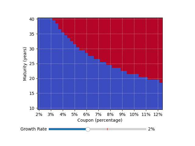
The red area indicates models with negative first principal payments.
I’m using some HTML and Javascript to generate the slider above, since matplotlib does’t play nicely with static websites. I learned how to make graphs with matplotlib over a decade ago, but it seems like plotly is much better nowadays. I didn’t want to rebuild my graph using plotly just to make the graph look nicer on this site simply because I wanted to get this blog post up already.
Analysis
A growth rate of 0% means we can extend the maturity out to 40 years regardless of our (reasonable choice of) coupon rate. That follows the result from my post on January 3rd. The more interesting cases involve growing revenues. With 2% annual growth, we can get out to about 30 years with coupons below about 6%.
In practice, we can fund some of the early interest costs from bond proceeds - you’ll see that referred to as capitalizing the interest. That means that we can get a little bit into the red in the graphs above by funding the deficit (i.e., the ‘negative principal payment’) up front.
The IRS limits tax-exempt bonds to three year’s worth of capitalized interest, however, so we can’t get too far into the red before we jeopardize the tax status of our muni bond. More practically, you don’t want to be capitalizing a bunch of interest if you can avoid it. It lowers how much in proceeds the issuer gets from the bond sale dollar-for-dollar, not to mention it just feels bad. Why are you borrowing money to pay the interest on the money you borrowed? A better tool in this situation is a Capital Appreciation Bond, the muni market equivalent of a zero coupon bond. This accretes the interest to the principal amount rather than needing to fund interest payments from bond proceeds.
Where on these graphs are most muni bonds? Well, most bonds are General Obligation Bonds with level debt service (i.e., no growth in debt service year over year). Those deals don’t need to worry about this analysis at all.
How about Revenue Bonds, especially in Project Finance? These deals will often structure debt service around some assumed revenue curve with some growth assumption built in. This is where I got the idea to do this analysis in the first place.
2% growth is a good estimate for the growth of most tax streams because it’s what the Fed targets for inflation. Sales taxes and income taxes are pretty clearly connected with inflation, and in many states property taxes are also limited to growing by inflation plus some fixed amount. So, most of the time we’re focused on that slide.
Most Project Finance deals have 25-30 year maturities, and most are sold non-rated with interest rates (in today’s market) around 5.50% to 6.50%. What we see in the graph above is that we should have no problem structuring fully amortizing bonds under these constraints.
However, when we push the growth rate up to 3% or higher, we start to run into problems that capitalized interest can’t handle.
Solutions for High Growth Rates and Coupons
The first tool issuers and their bankers reach for is capitalized interest. There’s usually a 1-3 year delay between issuance and when revenue is available to pay debt service anyways, during which the project is being built and stabilized. If there’s still space under the IRS 3-year limit, issuers can fund some of the interest upfront and delay paying principal by another year or two to make the model pencil.
When that doesn’t work, the next option to consider is a Capital Appreciation Bond (CAB). These can be set up as Convertible CABs which accrete interest until some predetermined date and then ‘convert’ into current interest bonds with regular interest payments. Anecdotally, I’ve seen this structure used in Colorado and Utah recently for single-family home developments which may have 4-5 year periods before sufficient absorption has occured to generate the property taxes needed to pay debt service.
In my experience, that’s the best tool available. Some borrowers don’t like the CAB structure because the interest accretion means the bonds are effectively sold with a steep discount to par. Some states place limitations on the discount at issuance, as well. When a CAB is ruled out, the last ditch resort is to revise the revenue projections: assume 2% growth instead of 3%, for example, and show investors the coverage ratio resulting from the higher growth rate to try to get a lower spread out of them.
Further Exploration
We’ve gone from no-growth revenue scenarios to steady growth rates. The natural next step would be to consider arbitrary revenue curves. This becomes analytically untractable quickly, so I’m switching gears.
For my next post, I’m planning to build a simple bond model app with Streamlit that lets you quickly mock up a bond model with some simplified assumptions. Version one will let the user quickly build models like the ones I’ve been working with in this post series, with fixed growth rate revenue curves. Version two will expand that to allow arbitrary revenue curves with automatically calculated capitalized interest. Stay tuned.