01 Feb 2026
The US dollar hit a four-year low this month following some, uh, interesting policy coming from the White House as well as comments from the president indicating he doesn’t really mind the currency weakness. The New York Fed performed a rate check in Yen markets, pretty much the only major currency that hasn’t been gaining on the dollar.
All of this has had me thinking more about currencies, one of the markets I know comparatively less about. One common way to display currency markets at a glance is a cross rates table showing conversion rates between major currencies. Here’s an example from Bloomberg.
While bored at work the other day, I played around with a graphical representation of that table. Here’s the basic idea:
- Suppose there are $n$ different currencies (I’ll use five in the examples below).
- Each currency pair has a conversion rate. Suppose the rate going from $A$ to $B$ is $r_{AB}$. Then the rate going from $B$ to $A$ is $r_{BA} = 1 / r_{AB}$.
- No arbitrage is enforced. That means there shouldn’t be a way to convert a unit of one currency to another at a rate higher or lower than the direct conversion rate. Mathematically, that means $r_{AC} = r_{AB} r_{BC}$, for example.
Using those rules, we can build a cross rates table with just $n-1$ cross rates; specifically, we only need the conversion rates from one currency to all of the others in order to get the rest of the rates. I’ll demonstrate by building the table.
I’ll represent the table as an $n$-by-$n$ matrix, where the $(i,j)$ entry gives us how much of currency $i$ is equal to 1 unit of currency $j$.
import numpy as np
from sympy import Matrix, init_printing
import matplotlib.pyplot as plt
import networkx as nx

rng = np.random.default_rng()
np.set_printoptions(suppress=True, precision=4)
# We'll work with just 5 currencies for legibility.
n = 5

# First, the conversion rate from a currency to itself is just one.
cross_rates = np.eye(n)
Matrix(cross_rates)
# Next, fill in our assumed conversion rates.
# These are actual conversion rates from USD to
# EUR, JPY, GBP, and CHF pulled on February 1st, 2026.
primary_conv_rates = np.asarray([0.8438, 154.7800, 0.7307, 0.7730])
cross_rates[1:, 0] = primary_conv_rates
Matrix(cross_rates)
# The rates from USD to those currencies are just the inverse of
# the rates from those currencies to USD.
cross_rates[0][1:] = 1 / primary_conv_rates

# I'm printing the matrix with decimals rounded to 4 places for legibility.
Matrix(cross_rates).applyfunc(lambda x: round(x, 4))
To fill in the rest of the table, we’ll take advantage of our third assumption. In order for there to be no arbitrage, it must be the case that $r_{BC} = r_{BA} r_{AC}$. Letting $A$ be USD, which is the currency whose cross rates we’re starting with, we can fill in the cross rates between other currencies by going through USD.
for i in range(2,n):
    for j in range (1,n-1):
        cross_rates[i][j] = cross_rates[i][0] * cross_rates[0][j]
        cross_rates[j][i] = 1 / cross_rates[i][j]

Matrix(cross_rates).applyfunc(lambda x: round(x, 4))
I used the networkx package to make a graph. Gemini is a great tool for people like myself, who have programming backgrounds but don’t do it every day. It made it really easy to find the right functions to use by just asking, “how do I do [x]?” and then looking the function up in the package’s documentation. I could probably have done this faster by describing exactly what I wanted to do to a thinking model, but doing it this way helped me learn the package.
# Generate the graph from the array.
G = nx.from_numpy_array(cross_rates, create_using=nx.DiGraph)
# By default, the nodes are named with integers.
# The below renames the nodes to the appropriate currencies.
node_names = ["USD","EUR","JPY","GBP","CHF"]
mapping = {i: name for i, name in enumerate(node_names)}
nx.relabel_nodes(G, mapping, copy=False)
# Remove self-edges (i.e., the conversion rate from a currency to itself)
# to make it easier to read.
G.remove_edges_from(nx.selfloop_edges(G))
# Set the layout of the nodes and generate the pyplot graph
pos = nx.circular_layout(G)
plt.figure(figsize=(8,8))
nx.draw(
G, pos, with_labels=True,
node_color='lightblue', node_size=700,
arrowsize=20, connectionstyle="arc3,rad=0.1"
)
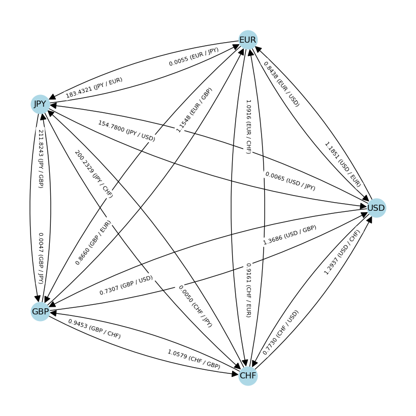
elabels = { (u, v): f"{d['weight']:.4f} ({u} / {v})" for u, v, d in G.edges(data=True) }
nx.draw_networkx_edge_labels(G, pos, edge_labels=elabels, label_pos=0.25, font_size=8)
plt.show()
You could compare the table generated from one currency’s exchange rates to actual market exchange rates. Since the table is constructed assuming no arbitrage, any differences between its predicted rates and market rates presumably represent arbitrage opportunities. This is something researchers actually do, as in this paper. From its abstract alone, you can immediately tell that the real world is much more complicated than this toy model, but it’s a useful framework all the same.